I get bored from doing two things: i) spot-checking + optimising parameters of my predictive models and ii) reading about how ‘black box’ machine learning (particularly deep learning) models are and how little we can do to better understand how they learn (or not learn, for example when they take a panda bear for a vulture!). In this post I’ll test a) H2O’s function h2o.automl() that may help me automate the former and b) Thomas Lin Pedersen’s library(lime) that may help clarify the latter.
ACCURATE & AUTOMATED PREDICTIVE MODELS USING h2o.automl()
This post would never happen if not for the inspiration I got from two excellent blog posts: Shirin Glander’s Lime presentation and Matt Dancho ‘s HR data analysis. There’s no hiding that this post is basically copy-catting their work - at least I’m standing on the shoulders of giants, hey!
I’ll use the powerful h2o.automl() function to optimise and choose the most accurate model classifying benign and malignant cancer cells from the Wisconsin dataset.
First, let’s load the data:
### loading cancer data ####
library(mlbench)

data(BreastCancer)
str(BreastCancer)
## 'data.frame':    699 obs. of  11 variables:
##  $ Id             : chr  "1000025" "1002945" "1015425" "1016277" ...
##  $ Cl.thickness   : Ord.factor w/ 10 levels "1"<"2"<"3"<"4"<..: 5 5 3 6 4 8 1 2 2 4 ...
##  $ Cell.size      : Ord.factor w/ 10 levels "1"<"2"<"3"<"4"<..: 1 4 1 8 1 10 1 1 1 2 ...
##  $ Cell.shape     : Ord.factor w/ 10 levels "1"<"2"<"3"<"4"<..: 1 4 1 8 1 10 1 2 1 1 ...
##  $ Marg.adhesion  : Ord.factor w/ 10 levels "1"<"2"<"3"<"4"<..: 1 5 1 1 3 8 1 1 1 1 ...
##  $ Epith.c.size   : Ord.factor w/ 10 levels "1"<"2"<"3"<"4"<..: 2 7 2 3 2 7 2 2 2 2 ...
##  $ Bare.nuclei    : Factor w/ 10 levels "1","2","3","4",..: 1 10 2 4 1 10 10 1 1 1 ...
##  $ Bl.cromatin    : Factor w/ 10 levels "1","2","3","4",..: 3 3 3 3 3 9 3 3 1 2 ...
##  $ Normal.nucleoli: Factor w/ 10 levels "1","2","3","4",..: 1 2 1 7 1 7 1 1 1 1 ...
##  $ Mitoses        : Factor w/ 9 levels "1","2","3","4",..: 1 1 1 1 1 1 1 1 5 1 ...
##  $ Class          : Factor w/ 2 levels "benign","malignant": 1 1 1 1 1 2 1 1 1 1 ...
.. and do some data cleaning: change column names, get rid of the order in factor levels and remove rows with empty cells:
### data pre-processing ####

library(dplyr)
library(janitor)
library(h2o)

bc_edited =
  BreastCancer %>%
  janitor::clean_names() %>% # changes dots in colnames to underscores
  mutate_if(is.factor, factor, ordered = FALSE) %>% # changes all columns to unordered factors
  select(class, everything(), -id) %>%
  na.omit()

str(bc_edited)
## 'data.frame':    683 obs. of  10 variables:
##  $ class          : Factor w/ 2 levels "benign","malignant": 1 1 1 1 1 2 1 1 1 1 ...
##  $ cl_thickness   : Factor w/ 10 levels "1","2","3","4",..: 5 5 3 6 4 8 1 2 2 4 ...
##  $ cell_size      : Factor w/ 10 levels "1","2","3","4",..: 1 4 1 8 1 10 1 1 1 2 ...
##  $ cell_shape     : Factor w/ 10 levels "1","2","3","4",..: 1 4 1 8 1 10 1 2 1 1 ...
##  $ marg_adhesion  : Factor w/ 10 levels "1","2","3","4",..: 1 5 1 1 3 8 1 1 1 1 ...
##  $ epith_c_size   : Factor w/ 10 levels "1","2","3","4",..: 2 7 2 3 2 7 2 2 2 2 ...
##  $ bare_nuclei    : Factor w/ 10 levels "1","2","3","4",..: 1 10 2 4 1 10 10 1 1 1 ...
##  $ bl_cromatin    : Factor w/ 10 levels "1","2","3","4",..: 3 3 3 3 3 9 3 3 1 2 ...
##  $ normal_nucleoli: Factor w/ 10 levels "1","2","3","4",..: 1 2 1 7 1 7 1 1 1 1 ...
##  $ mitoses        : Factor w/ 9 levels "1","2","3","4",..: 1 1 1 1 1 1 1 1 5 1 ...
##  - attr(*, "na.action")=Class 'omit'  Named int [1:16] 24 41 140 146 159 165 236 250 276 293 ...
##   .. ..- attr(*, "names")= chr [1:16] "24" "41" "140" "146" ...
That’s better! Now, let’s set up the local H2O instance…
h2o.init() # initializes Java Virtual Machine (JVM)
##  Connection successful!
##
## R is connected to the H2O cluster:
##     H2O cluster uptime:         7 hours 8 minutes
##     H2O cluster version:        3.14.0.3
##     H2O cluster version age:    1 month and 16 days
##     H2O cluster name:           H2O_started_from_R_katarzynakulma_ihv753
##     H2O cluster total nodes:    1
##     H2O cluster total memory:   0.11 GB
##     H2O cluster total cores:    4
##     H2O cluster allowed cores:  4
##     H2O cluster healthy:        TRUE
##     H2O Connection ip:          localhost
##     H2O Connection port:        54321
##     H2O Connection proxy:       NA
##     H2O Internal Security:      FALSE
##     H2O API Extensions:         XGBoost, Algos, AutoML, Core V3, Core V4
##     R Version:                  R version 3.3.3 (2017-03-06)
h2o.no_progress() # Turn off output of progress bars
… and split the data into training, validation and testing datasets.
bc_h2o <- as.h2o(bc_edited)

split_h2o <- h2o.splitFrame(bc_h2o, c(0.7, 0.15), seed = 13 ) #splits data into random 70%/15%15% chunks

train_h2o <- h2o.assign(split_h2o[[1]], "train" ) # 70%
valid_h2o <- h2o.assign(split_h2o[[2]], "valid" ) # 15%
test_h2o  <- h2o.assign(split_h2o[[3]], "test" )  # 15%
Finally, we can now use the famous h2o.automl() function and set the model up: set the target, feature names, training and validation sets, as well as how long we want the algorithm to run for (for this you can use either max_runtime_secs argument, like I did here, or max_models, see h2o.automl() documentation for details.
# Sets target and feature names for h2o
y <- "class"
x <- setdiff(names(train_h2o), y)

# Run the automated machine learning
models_h2o <- h2o.automl(
  x = x, # predictors
  y = y, # labels
  training_frame    = train_h2o, # training set
  leaderboard_frame = valid_h2o, # validation set
  max_runtime_secs  = 60 # run-time can be increased/decreased according to your needs
)
The algorithm will run random forest (RF), gradient boosting machines (GBM), generalised linear models (GLM) and deep learning (DL) models. It will then produce a leaderboard based on the best stopping metric (which you can choose by defining stopping_metric parameter). For more details see this chapter from Practical Machine Learning with H2O by Darren Cook. You can see the best model by picking up a @leader.
### leaderboard

lb <- models_h2o@leaderboard
lb
##                                    model_id      auc  logloss
## 1     DeepLearning_0_AutoML_20171107_162913 0.996622 0.081152
## 2     DeepLearning_0_AutoML_20171107_230040 0.994932 0.090049
## 3 GBM_grid_1_AutoML_20171107_162650_model_1 0.994088 0.637539
## 4 GBM_grid_1_AutoML_20171107_170043_model_6 0.993243 0.101251
## 5 GBM_grid_1_AutoML_20171107_230502_model_0 0.993243 0.104345
## 6 GBM_grid_0_AutoML_20171107_170043_model_4 0.992821 0.107482
##
## [402 rows x 3 columns]
Neural network wins, followed by gradient boost models - no surprise here!
Finally, you can use the Leader to predict labels of the testing set:
automl_leader <- models_h2o@leader

h20_pred <- h2o.predict(automl_leader, test_h2o)
It IS that easy, no joke. Let’s have a quick look at the confusion matrix…
library(tibble)

test_performance <- test_h2o %>%
  tibble::as_tibble() %>%
  select(class) %>%
  tibble::add_column(prediction = as.vector(h20_pred$predict)) %>%
  mutate(correct = ifelse(class == prediction, "correct", "wrong")) %>%
  mutate_if(is.character, as.factor)

head(test_performance)
## # A tibble: 6 x 3
##       class prediction correct
##      <fctr>     <fctr>  <fctr>
## 1    benign     benign correct
## 2    benign     benign correct
## 3 malignant     benign   wrong
## 4    benign     benign correct
## 5 malignant  malignant correct
## 6 malignant  malignant correct
confusion_matrix <- test_performance %>% select(-correct) %>% table()
confusion_matrix
##            prediction
## class       benign malignant
##   benign        61         1
##   malignant      5        33
… and more detailed performance of the model.
#### Performance analysis ####
tn <- confusion_matrix[1]
tp <- confusion_matrix[4]
fp <- confusion_matrix[3]
fn <- confusion_matrix[2]

accuracy <- (tp + tn) / (tp + tn + fp + fn)
misclassification_rate <- 1 - accuracy
recall <- tp / (tp + fn)
precision <- tp / (tp + fp)
null_error_rate <- tn / (tp + tn + fp + fn)

library(purrr)

tibble(
  accuracy,
  misclassification_rate,
  recall,
  precision,
  null_error_rate
) %>%
  purrr::transpose()
## [[1]]
## [[1]]$accuracy
## [1] 0.94
##
## [[1]]$misclassification_rate
## [1] 0.06
##
## [[1]]$recall
## [1] 0.8684211
##
## [[1]]$precision
## [1] 0.9705882
##
## [[1]]$null_error_rate
## [1] 0.61
Given that it is cancer data I’d be happier if recall was higher, but longer running times would improve this. Now, can we understand the neural network - the king of ‘black-box’ learners - that produced those predictions?
MAKING OBSCURE LESS OBSCURE USING library(lime)
The answer is (to certain extend) YES and package lime will help us with it. Following Shirin’s example, I’ll split the data into correct and wrong predictions to better understand what confused the model about misclassified observations.
test_h2o_df = as.data.frame(test_h2o)

test_h2o_2 = test_h2o_df %>%
  as.data.frame() %>%
  mutate(sample_id = rownames(test_h2o_df ))

test_correct <- test_performance %>%
  mutate(sample_id = rownames(test_performance)) %>%
  filter(correct == 'correct') %>%
  inner_join(test_h2o_2) %>%
  select(-c(prediction, correct, sample_id))

test_wrong <- test_performance %>%
  mutate(sample_id = rownames(test_performance)) %>%
  filter(correct == 'wrong') %>%
  inner_join(test_h2o_2) %>%
  select(-c(prediction, correct, sample_id))
Now, let’s prepare lime so that it works with H2O model correctly. No one will explain this step better than Matt (the author) himself:
The
limepackage implements LIME in R. One thing to note is that it’s not setup out-of-the-box to work with h2o. The good news is with a few functions we can get everything working properly. We’ll need to make two custom functions:
model_type: Used to tell lime what type of model we are dealing with. It could be classification, regression, survival, etc.
predict_model: Used to allow lime to perform predictions that its algorithm can interpret.
library(lime)

# Setup lime::model_type() function for h2o
model_type.H2OBinomialModel <- function(x, ...) {
  return("classification")
}

# Setup lime::predict_model() function for h2o
predict_model.H2OBinomialModel <- function(x, newdata, type, ...) {
  pred <- h2o.predict(x, as.h2o(newdata))
  # return probs
  return(as.data.frame(pred[,-1]))
}
We’re nearly there! Let’s just define our explainer…
predict_model(x = automl_leader, newdata = as.data.frame(test_h2o[,-1]), type = 'raw') %>%
  tibble::as_tibble()
## # A tibble: 100 x 2
##        benign    malignant
##         <dbl>        <dbl>
##  1 0.99912117 0.0008788323
##  2 0.99911889 0.0008811068
##  3 0.86410812 0.1358918824
##  4 0.99884181 0.0011581938
##  5 0.02542826 0.9745717393
##  6 0.01327680 0.9867232037
##  7 0.02752797 0.9724720317
##  8 0.80216260 0.1978373974
##  9 0.99859496 0.0014050448
## 10 0.99271180 0.0072882030
## # ... with 90 more rows
explainer <- lime::lime(
  as.data.frame(train_h2o[,-1]),
  model          = automl_leader,
  bin_continuous = FALSE)
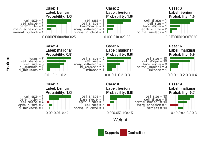
… and let’s start explaining! All our work so far lead to this feature importance plots (not the same for each case!). The green bars mean that the feature supports predicted label, and the red bars contradict it. Let’s have a look at the correctly predicted labels:
explanation_corr <- explain(
  test_correct[1:9, -1],
  explainer = explainer,
  n_labels = 1,
  n_features = 5,
  kernel_width = 0.5)

plot_features(explanation_corr, ncol = 3)

You can see that smaller and more regular cells with low values of bare nuclei (bare_nuclei) correctly indicate benign cells, whereas big, irregular cells with higher values of clump thickness (cl_thickness) support malignant label. It all makes sense.
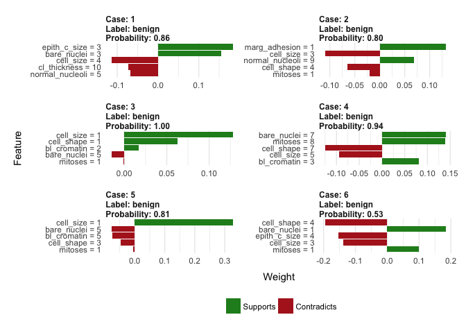
What about the misclasified labels?
explanation_wrong <- explain(
  test_wrong[1:6, -1],
  explainer = explainer,
  n_labels = 1,
  n_features = 5,
  kernel_width = 0.5)

plot_features(explanation_wrong)

And here’s where the true power of lime package is: understanding what made model missclasify labels. All the wrong cases were predcited to be benign while they were malignant, why? It looks like they were mainly small and quite regular cells, altough some malignant characterstics were still present (e.g. higher values of bare nuclei and clump thickness). What a great improvement of our understanding of how the ‘black box’ model works and why it makes mistakes. Even though it doesn’t produce ‘fixed’ feature importance plots (i.e. a general, not case-to-case view of which variables are most informative when making a prediction), it allows you to make a good educated guess of which features matter. We live in beautiful times!