It will go without saying that I’m super excited about the premiere of another Star Wars movie and I’m not an exception. This, together with with Piotr Migdal’s challenge posted on Data Science PL group on Facebook where he suggested comparing word frequencies between two different sources. It didn’t take me long to decide what source to choose! So in this short kand sweer blogpost I’m comparing word frequencies between two movie scripts: “Star Wars: The New Hope” (1977) and “Star Trek: The Motion Picture” (1979). I chose these two because of 1) the obvious “competition” going on between the two camps and 2) similar time they were first broadcast. Let’s get cracking!
Let’s load necessary packages:
library(rvest)
library(dplyr)
## Warning: package 'dplyr' was built under R version 3.4.2
library(tm)
library(tidytext)
## Warning: package 'tidytext' was built under R version 3.4.2
library(ggthemes)
library(ggplot2)
library(DT)
The first one, rvest, comes in handy in web-scraping text from the movie scripts (it’s amazing what you can get online for free these days):
swIV_url <-"http://www.imsdb.com/scripts/Star-Wars-A-New-Hope.html"
startrek_url <- "http://www.dailyscript.com/scripts/startrek01.html"

star_wars <- read_html(swIV_url) %>%
  html_nodes("td") %>%
  html_text() %>%
  .[[88]]

star_trek <- read_html(startrek_url) %>%
  html_nodes("pre") %>%
  html_text()

str(star_wars)
## chr "\r\n\r\n\n\n\n STAR WARS\n\n Epis"| __truncated__
As you can see, the script texts are very messy, so I write a customised function to clean them up a bit:
clean_text <- function(x) {
  x <- gsub("\\\n", " ", x)
  x <- gsub("\\\r", " ", x)
  x <- gsub("\\\t", " ", x)
  x <- gsub("[[:punct:]]", " ", x)
  x <- x %>%
    tolower() %>%
    removeNumbers() %>%
    stripWhitespace()
  x}


clean_star_trek <- clean_text(star_trek)
clean_star_wars <- clean_text(star_wars)

str(clean_star_wars)
## chr " star wars episode iv a new hope from the journal of the whills by george lucas revised fourth draft january lu"| __truncated__
That’s MUCH better! From here, we are only a few steps away from getting the desired word frequency tables:
data("stop_words")


sw_tokens <- clean_star_wars %>%
  as_tibble() %>% # trasforming vector to tibble
  rename_(sw_text = names(.)[1]) %>% # assign a column name
  mutate_if(is.factor, as.character) %>% # convert it from factor to character
  mutate(swt=unlist(sw_text)) %>%
  unique() %>%
  unnest_tokens("word", sw_text) %>% # break text down into single words
  anti_join(stop_words) %>% # remove stop words
  count(word, sort = TRUE) %>% # count word frequency and sort it in decreasing order
  rename(sw_n = n)


st_tokens <- clean_star_trek %>%
  as_tibble() %>%
  rename_(st_text = names(.)[1]) %>%
  mutate_if(is.factor, as.character) %>%
  mutate(stt=unlist(st_text)) %>%
  unique() %>%
  unnest_tokens("word", st_text) %>%
  anti_join(stop_words) %>%
  count(word, sort = TRUE) %>%
  rename(st_n = n)

sw_tokens
## # A tibble: 3,385 x 2
##        word  sw_n
##       <chr> <int>
##  1     luke   726
##  2      int   314
##  3      han   269
##  4     star   235
##  5    death   229
##  6 threepio   217
##  7  cockpit   196
##  8      ben   176
##  9      ext   167
## 10    vader   162
## # ... with 3,375 more rows
TA-DA! Our tables are ready and squeky clean :) Now, I’ll use inner_join() to narrow down the data to only those words that the two scripts have in common. To compare the frequencies I’ll use a variable called log_word_prop: logarithm of the proportion between Star Wars and Star Trek word frequency. This means that the more positive the value, the more drastic the difference in frequency it is in favour of Star Wars. On the other hand, the more negative the value, the more commonly it was used in Star Trek (in comparison to Star Wars).
final_tokens = sw_tokens %>%
  inner_join(st_tokens) %>%
  mutate(log_word_prop =  round(log(sw_n / st_n),3),
         dominates_in = as.factor(ifelse(log_word_prop > 0, "star_wars", "star_trek")))

final_tokens
## # A tibble: 1,293 x 5
##       word  sw_n  st_n log_word_prop dominates_in
##      <chr> <int> <int>         <dbl>       <fctr>
##  1     int   314   110         1.049    star_wars
##  2    star   235     9         3.262    star_wars
##  3   death   229     1         5.434    star_wars
##  4     ext   167    49         1.226    star_wars
##  5     red   152     7         3.078    star_wars
##  6 fighter   121     1         4.796    star_wars
##  7    wing   112     1         4.718    star_wars
##  8    ship   109    48         0.820    star_wars
##  9   space    90    45         0.693    star_wars
## 10 surface    87     5         2.856    star_wars
## # ... with 1,283 more rows
And we can finally visualise our findings: first, let’s have a quick glipse on what words occured in pretty much the same frequency in both movies:
set.seed(13)

final_tokens %>%
  filter(abs(log_word_prop) == 0) %>%
  arrange(desc(sw_n)) %>%
  sample_n(30) %>%
  ggplot(aes(x = reorder(word, log_word_prop),  y = log_word_prop, fill = dominates_in)) +
  geom_bar(stat  = "identity", show.legend = FALSE) +
  theme_minimal() +
  coord_flip() +
  xlab("") +
  ylab("log(word_prop)") +
  scale_fill_brewer(palette = "Set1") +
  ggtitle("Sample of words that occur with the same frequency in SW and ST")
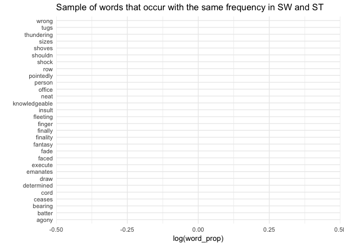
I must say, I expected this most similar vocabulary to be much more technical. At the same time, this time according to expectations, those words reflect action and drama in both movies: things cease, emanate and shove, people shock, experience agony and are determined and knowledgeable.
What about most polarizing words? I chose to show the words that were at least 12 times (log_word_prop > 2.4) more common in one movie than the other. What are they?
final_tokens %>%
  filter(abs(log_word_prop) > 2.4) %>%
  filter(!word %in% c("ext", "int")) %>%
  ggplot(aes(x = reorder(word, log_word_prop),  y = log_word_prop, fill = dominates_in)) +
  geom_bar(stat  = "identity") +
  theme_minimal() +
  coord_flip() +
  xlab("") +
  ylab("log(word_prop)") +
  scale_fill_brewer(palette = "Set1") +
  ggtitle("Words that show strikingly different frequencies in Star Wars and Star Trek")
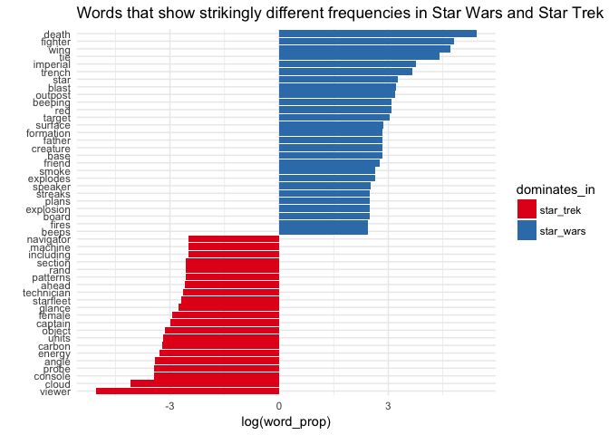
Haha! You may not be surprised that the most Star Wars-y vocabulary is full of words like death, star, imperial or even father, but I didn’t expect female or cloud to be THAT much more present in Star Trek! Some things never cease to surprise even most determined and knowledgeable people, even if they have assistance of imperial technician ;-)
UPDATE!!
After Piotr’s suggestion, I decided to play a bit with ggplot’s excellent geom_text(). This little tweak can give you surprising inisghts into the Word Battle matter! Below I plotted the more dominant frequency of a given word againts a relative difference in word proportion:
final_tokens %>%
  mutate(dominant_freq = as.numeric(ifelse(sw_n > st_n, sw_n, st_n))) %>%
  filter(!word %in% c("ext", "int")) %>%
  ggplot(aes(log_word_prop, dominant_freq, label = word)) +
  geom_text(check_overlap = TRUE) +
  theme_minimal() +
  ylab("Word frequency in a dominating movie") +
  xlab("log(word_prop)") +
  scale_fill_brewer(palette = "Set1") +
  ggtitle("Word frequency by word proportion in Star Wars and Star Trek")
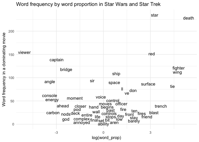
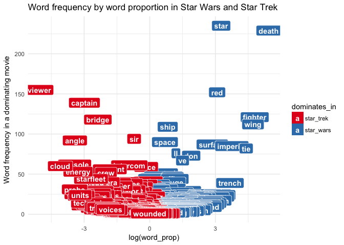
Not a bad start! A much more appealing - although a bit less readable - look can be achieved with geom_label():
final_tokens %>%
  mutate(dominant_freq = as.numeric(ifelse(sw_n > st_n, sw_n, st_n))) %>%
  filter(!word %in% c("ext", "int")) %>%
  ggplot(aes(log_word_prop, dominant_freq, label = word)) +
  geom_label(aes(fill = dominates_in), colour = "white", fontface = "bold") +
  theme_minimal() +
  ylab("Word frequency in a dominating movie") +
  xlab("log(word_prop)") +
  scale_fill_brewer(palette = "Set1") +
  ggtitle("Word frequency by word proportion in Star Wars and Star Trek")