Have you ever wondered whether the most active/popular R-twitterers are virtual friends? :) And by friends here I simply mean mutual followers on Twitter. In this post, I score and pick top 30 #rstats twitter users and analyse their Twitter friends’ network. You’ll see a lot of applications of rtweet and ggraph packages, as well as a very useful twist using purrr library, so let’s begin!
BEFORE I START: OFF - TOPIC ON PERFECTIONISM
After weeks and months (!!!) of not publishing anything, finally this post sees the light of day! It went through so many tests and changes - including conceptual ones! - that I’m relieved now that it’s out and I can move on to another project. But I learned my lesson: perfectionism can be a real hurdle for any developer/data scientist and clearly, I’m not alone with this experience. So, next time I’m not going to take that long to push something out - imperfect projects can improve and refine once they’re out and I suppose they engage more people by provoking them to give ideas and suggest better solutions. Anyway, where were we…? :)
IMPORTING #RSTATS USERS
After loading my precious packages…
library(rtweet)
library(dplyr)
library(purrr)
library(igraph)
library(ggraph)
… I searched for Twitter users that have rstats in their profile description. It definitely doesn’t include ALL active and popular R - users, but it’s a pretty reliable way of picking definite R - fans.
r_users <- search_users("#rstats", n = 1000)
It’s important to say, that in rtweet::search_users() even if you specify 1000 users to be extracted, I ended up with quite a few duplicates and the actual number of users I got was much smaller: 565
r_users %>% summarise(n_users = n_distinct(screen_name))
##   n_users
## 1     564
Funnily enough, even though my profile description contains #rstats, I was not included in the search results (@KKulma), sic! Were you? :)
r_users %>% select(screen_name) %>% unique() %>% arrange(screen_name) %>% DT::datatable()
plot of chunk sorted_users
SCORING AND CHOOSING TOP #RSTATS USERS
Now, let’s extract some useful information about those users:
r_users_info <- lookup_users(r_users$screen_name)
You’ll notice, that created data frame holds information about number of followers, friends (users they follow), lists they belong to, number of tweets (statuses) or how many times sometimes marked those tweets as their favourite.
r_users_info %>% select(dplyr::contains("count")) %>% head()
##   followers_count friends_count listed_count favourites_count
## 1            8311           366          580             9325
## 2           44474            11         1298                3
## 3           11106           524          467            18495
## 4           12481           431          542             7222
## 5           15345          1872          680            27971
## 6            5122           700          549             2796
##   statuses_count
## 1          66117
## 2           1700
## 3           8853
## 4           6388
## 5          22194
## 6          10010
And these variables I use for building my ‘top score’: I simply calculate a percentile for each of those variables and sum it altogether. Given that each variable’s percentile will give me a value between 0 and 1, The final score can have a maximum value of 5.
r_users_ranking <- r_users_info %>%
  filter(protected == FALSE) %>%
  select(screen_name, dplyr::contains("count")) %>%
  unique() %>%
  mutate(followers_percentile = ecdf(followers_count)(followers_count),
         friends_percentile = ecdf(friends_count)(friends_count),
         listed_percentile = ecdf(listed_count)(listed_count),
         favourites_percentile = ecdf(favourites_count)(favourites_count),
         statuses_percentile = ecdf(statuses_count)(statuses_count)
         ) %>%
  group_by(screen_name) %>%
  summarise(top_score = followers_percentile + friends_percentile + listed_percentile + favourites_percentile + statuses_percentile) %>%
  ungroup() %>%
  mutate(ranking = rank(-top_score))
All I need to do now is to pick top 30 users based on the score I calculated. Did you manage get onto the top 30 list? :)
top_30 <- r_users_ranking %>% arrange(desc(top_score)) %>% head(30) %>% arrange(desc(top_score))
top_30 %>% as.data.frame() %>% select(screen_name) %>% DT::datatable()
plot of chunk top_30
I must say I’m incredibly impressed by these scores: @hpster, THE top R - twitterer managed to obtain a score of over 4.8 out of 5! Also, @Physical_Prep and @TheSmartJokes managed to tie 8th place, which I thought was unlikely to happed, given how granular the score is.
Anyway! To add some more depth to my list, I tried to identify those users’ gender, to see how many top users are women. I had to do it manually (sic!), as the Twitter API’s data doesn’t provide this, AFAIK. Let me know if you spot any mistakes!
top30_lookup <- r_users_info %>%
  filter(screen_name %in% top_30$screen_name) %>%
  select(screen_name, user_id)

top30_lookup$gender <- c("M", "F", "F", "F", "F",
                         "M", "M", "M", "F", "F",
                         "F", "M", "M", "M", "F",
                         "F", "M", "M", "M", "M",
                         "M", "M", "M", "F", "M",
                         "M", "M", "M", "M", "M")

table(top30_lookup$gender)
##
##  F  M
## 10 20
It looks like a third of all top users are womes, but in the top 10 users there are 6 women. Better than I expected, actually. So, well done, ladies!
GETTING FRIENDS NETWORK
Now, this was the trickiest part of this project: extracting top users’ friends list and putting it all in one data frame. As you ma be aware, Twitter API has a limit od downloading information on 15 accounts in 15 minutes. So for my list, I had to break it up into 2 steps, 15 users each and then I named each list according to the top user they refer to:
top_30_usernames <- top30_lookup$screen_name

friends_top30a <-   map(top_30_usernames[1:15 ], get_friends)
names(friends_top30a) <- top_30_usernames[1:15]

# 15 minutes later....
friends_top30b <- map(top_30_usernames[16:30], get_friends)
After this I end up with two lists, each containing all friends’ IDs for top and bottom 15 users respectively. Here’s an example:
str(friends_top30b)
## List of 15
##  $ modernscientist:'data.frame':	1752 obs. of  1 variable:
##   ..$ user_id: chr [1:1752] "18153864" "19187806" "2785337469" "586883143" ...
##   ..- attr(*, "next_cursor")= chr "0"
##  $ Physical_Prep  :'data.frame':	2390 obs. of  1 variable:
##   ..$ user_id: chr [1:2390] "62836649" "228664938" "1941843097" "2523165143" ...
##   ..- attr(*, "next_cursor")= chr "0"
##  $ BillPetti      :'data.frame':	1140 obs. of  1 variable:
##   ..$ user_id: chr [1:1140] "119802433" "109303284" "482232051" "49155222" ...
##   ..- attr(*, "next_cursor")= chr "0"
##  $ JonathanAFrye  :'data.frame':	2611 obs. of  1 variable:
##   ..$ user_id: chr [1:2611] "34006491" "23342797" "64229716" "75051887" ...
##   ..- attr(*, "next_cursor")= chr "0"
##  $ ChetanChawla   :'data.frame':	1365 obs. of  1 variable:
##   ..$ user_id: chr [1:1365] "3362913279" "851583986270957568" "449588356" "15227791" ...
##   ..- attr(*, "next_cursor")= chr "0"
##  $ rogierK        :'data.frame':	1359 obs. of  1 variable:
##   ..$ user_id: chr [1:1359] "4427052929" "3315236924" "2976444713" "3865005196" ...
##   ..- attr(*, "next_cursor")= chr "0"
##  $ AriBFriedman   :'data.frame':	1414 obs. of  1 variable:
##   ..$ user_id: chr [1:1414] "805181039245225984" "740985271026491392" "2534410031" "720675478193971200" ...
##   ..- attr(*, "next_cursor")= chr "0"
##  $ yrochat        :'data.frame':	533 obs. of  1 variable:
##   ..$ user_id: chr [1:533] "2827803498" "311905244" "74398697" "3645507015" ...
##   ..- attr(*, "next_cursor")= chr "0"
##  $ TheSmartJokes  :'data.frame':	5000 obs. of  1 variable:
##   ..$ user_id: chr [1:5000] "891529978201780224" "811251016410664960" "891556417739608064" "843245938449833984" ...
##   ..- attr(*, "next_cursor")= chr "1545261800668264448"
##  $ mikkopiippo    :'data.frame':	4860 obs. of  1 variable:
##   ..$ user_id: chr [1:4860] "770326630145282048" "703923734" "49542761" "122129148" ...
##   ..- attr(*, "next_cursor")= chr "0"
##  $ rtraborn       :'data.frame':	1073 obs. of  1 variable:
##   ..$ user_id: chr [1:1073] "369101147" "81882372" "2639088547" "33867913" ...
##   ..- attr(*, "next_cursor")= chr "0"
##  $ b_prasad26     :'data.frame':	2426 obs. of  1 variable:
##   ..$ user_id: chr [1:2426] "75321229" "15851807" "484023344" "177444328" ...
##   ..- attr(*, "next_cursor")= chr "0"
##  $ ozjimbob       :'data.frame':	980 obs. of  1 variable:
##   ..$ user_id: chr [1:980] "17707546" "804157677177868288" "916685508" "2546258378" ...
##   ..- attr(*, "next_cursor")= chr "0"
##  $ ricobert1      :'data.frame':	707 obs. of  1 variable:
##   ..$ user_id: chr [1:707] "88731801" "153234994" "19878055" "2743609942" ...
##   ..- attr(*, "next_cursor")= chr "0"
##  $ PlethodoNick   :'data.frame':	1961 obs. of  1 variable:
##   ..$ user_id: chr [1:1961] "42486688" "15576928" "2154127088" "337318821" ...
##   ..- attr(*, "next_cursor")= chr "0"
So what I need to do now is i) append the two lists, ii) create a variable stating top users’ name in each of those lists and iii) turn lists into data frames. All this can be done in 3 lines of code. And brace yourself: here comes the purrr trick I’ve been going on about! Simply using purrr:::map2_df I can take a single list of lists, create a name variable in each of those lists based on the list name (twitter_top_user) and convert the result into the data frame. BRILLIANT!!
# turning lists into data frames and putting them together
friends_top30 <- append(friends_top30a, friends_top30b)
names(friends_top30) <- top_30_usernames

# purrr - trick I've been banging on about!
friends_top <- map2_df(friends_top30, names(friends_top30), ~ mutate(.x, twitter_top_user = .y)) %>%
  rename(friend_id = user_id) %>% select(twitter_top_user, friend_id)

# are we missing any users?
friends_top %>% summarize(dist = n_distinct(twitter_top_user))
##   dist
## 1   30
Here’s the last bit that I need to correct before we move to plotting the friends networks: for some reason, using purrr::map() with rtweet:::get_friends() gives me only 5000 friends, whereas the true value is over 8000. As it’s the only top user with more than 5000 friends, I’ll download his friends separately…
# getting a full list of friends
SJ1 <- get_friends("TheSmartJokes")
SJ2 <- get_friends("TheSmartJokes", page = next_cursor(SJ1))

# putting the data frames together
SJ_friends <-rbind(SJ1, SJ2) %>%
  rename(friend_id = user_id) %>%
  mutate(twitter_top_user = "TheSmartJokes") %>%
  select(twitter_top_user, friend_id)

# the final results - over 8000 friends, rather than 5000
str(SJ_friends)
## 'data.frame':	0 obs. of  2 variables:
##  $ twitter_top_user: chr
##  $ friend_id       : chr
… and use it to replace those that are already in the final friends list.
friends_top30 <- friends_top %>%
  filter(twitter_top_user != "TheSmartJokes") %>%
  rbind(SJ_friends)
Some final data cleaning: filtering out friends that are not among the top 30 R - users, replacing their IDs with twitter names and adding gender for top users and their friends… Tam, tam, tam: here we are! Here’s the final data frame we’ll use for visualising the friends networks!
# select friends that are top30 users
final_friends_top30 <- friends_top  %>%
  filter(friend_id %in% top30_lookup$user_id)

# add friends' screen_name
final_friends_top30$friend_name <- top30_lookup$screen_name[match(final_friends_top30$friend_id, top30_lookup$user_id)]

# add users' and friends' gender
final_friends_top30$user_gender <- top30_lookup$gender[match(final_friends_top30$twitter_top_user, top30_lookup$screen_name)]
final_friends_top30$friend_gender <- top30_lookup$gender[match(final_friends_top30$friend_name, top30_lookup$screen_name)]

## final product!!!
final <- final_friends_top30 %>% select(-friend_id)

head(final)
##   twitter_top_user     friend_name user_gender friend_gender
## 1         hrbrmstr nicoleradziwill           M             F
## 2         hrbrmstr        kara_woo           M             F
## 3         hrbrmstr      juliasilge           M             F
## 4         hrbrmstr        noamross           M             M
## 5         hrbrmstr      JennyBryan           M             F
## 6         hrbrmstr     thosjleeper           M             M
VISUALIZATING FRIENDS NETWORKS
After turning our data frame into something more usable by igraph and ggraph…
f1 <- graph_from_data_frame(final, directed = TRUE, vertices = NULL)
V(f1)$Popularity <- degree(f1, mode = 'in')
… let’s have a quick overview of all the connections:
ggraph(f1, layout='kk') +
  geom_edge_fan(aes(alpha = ..index..), show.legend = FALSE) +
  geom_node_point(aes(size = Popularity)) +
  theme_graph( fg_text_colour = 'black')
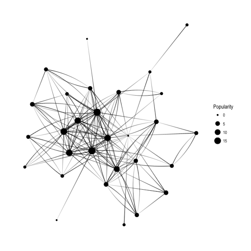
Keep in mind that Popularity - defined as the number of edges that go into the node - determines node size. It’s all pretty, but I’d like to see how nodes correspond to Twitter users’ names:
ggraph(f1, layout='kk') +
  geom_edge_fan(aes(alpha = ..index..), show.legend = FALSE) +
  geom_node_point(aes(size = Popularity)) +
  geom_node_text(aes(label = name, fontface='bold'),
                 color = 'white', size = 3) +
  theme_graph(background = 'dimgray', text_colour = 'white',title_size = 30)
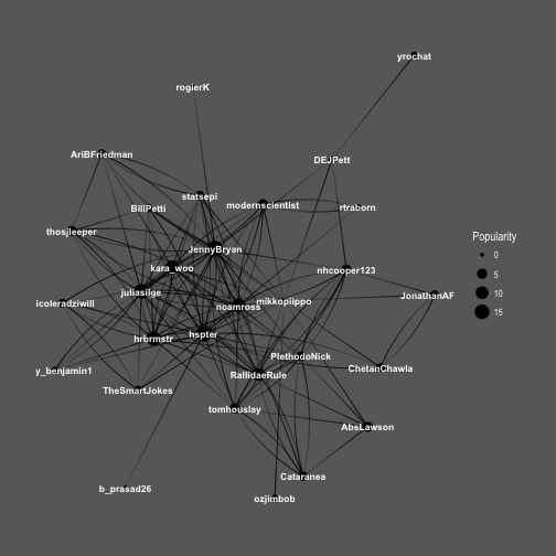
So interesting! You see the core of the graph consisting of mainly female users: @hpster, @JennyBryan, @juliasilge, @karawoo, but also a couple of male R - users: @hrbrmstr and @noamross. Who do they follow? Men or women?
ggraph(f1, layout='kk') +
  geom_edge_fan(aes(alpha = ..index..), show.legend = FALSE) +
  geom_node_point(aes(size = Popularity)) +
  theme_graph( fg_text_colour = 'black') +
  geom_edge_link(aes(colour = friend_gender)) +
  scale_edge_color_brewer(palette = 'Set1') +
  labs(title='Top 30 #rstats users and gender of their friends')
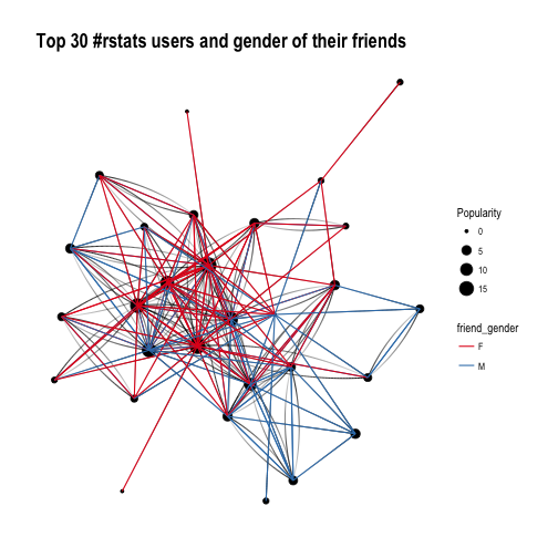
It’s difficult to say definitely, but superficially I see A LOT of red, suggesting that our top R - users often follow female top twitterers. Let’s have a closer look and split graphs by user gender and see if there’s any difference in the gender of users they follow:
ggraph(f1, layout='kk') +
  geom_edge_fan(aes(alpha = ..index..), show.legend = FALSE) +
  geom_node_point(aes(size = Popularity)) +
  theme_graph( fg_text_colour = 'black') +
  facet_edges(~user_gender) +
  geom_edge_link(aes(colour = friend_gender)) +
  scale_edge_color_brewer(palette = 'Set1') +
  labs(title='Top 30 #rstats users and gender of their friends', subtitle='Graphs are separated by top user gender, edge colour indicates their friend gender' )
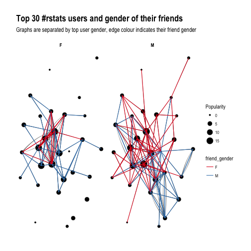
Ha! look at this! Obviously, Female users’ graph will be less dense as there are fewer of them in the dataset, however, you can see that they tend to follow male users more often than male top users do. Is that impression supported by raw numbers?
final %>%
  group_by(user_gender, friend_gender) %>%
  summarize(n = n()) %>%
  group_by(user_gender) %>%
  mutate(sum = sum(n),
         percent = round(n/sum, 2))
## # A tibble: 4 x 5
## # Groups:   user_gender [2]
##   user_gender friend_gender     n   sum percent
##         <chr>         <chr> <int> <int>   <dbl>
## 1           F             F    26    57    0.46
## 2           F             M    31    57    0.54
## 3           M             F    55   101    0.54
## 4           M             M    46   101    0.46
It looks so, although to the lesser extend than suggested by the network graphs: Female top users follower other female top users 46% of time, whereas male top users follow female top user 54% of time. So what do you have to say about that?