I’ve been writing/talking a lot about LIME] recently: in this blog/ at H20 meetup, or at coming AI Congress and I’m still sooo impressed by this tool for interpreting any, even black-box - algorithm! The part I love most is that LIME can be applied to both image and text data, that was well showcased in husky VS wolf (image) and Christian VS atheist (text) examples in the original publication. Thomas Lin Pedersen did an amazing job building lime package for R with excellent documentation and vignette. In fact, the lime vignette inspired a big part of this post. As you’ll soon see, lime keeps on giving when it comes to text classification. What do you say for classifying Clinton and Trump tweets?
As always, let’s start with loading necessary packages.
library(readr)
library(lime)
library(xgboost) # the classifier
library(caret)
library(dplyr)
library(tibble)
library(text2vec)
library(qdapRegex) # removes urls from text
Next, let’s load the data that was kindly provided on Kaggle.
tweets <- read_csv('data/tweets.csv')
dim(tweets)
## [1] 6444 28
head(tweets)
## # A tibble: 6 x 28
##             id          handle
##          <dbl>           <chr>
## 1 7.809256e+17  HillaryClinton
## 2 7.809162e+17  HillaryClinton
## 3 7.809116e+17  HillaryClinton
## 4 7.809070e+17  HillaryClinton
## 5 7.808974e+17  HillaryClinton
## 6 7.808931e+17 realDonaldTrump
## # ... with 26 more variables: text <chr>, is_retweet <chr>,
## #   original_author <chr>, time <dttm>, in_reply_to_screen_name <chr>,
## #   in_reply_to_status_id <dbl>, in_reply_to_user_id <dbl>,
## #   is_quote_status <chr>, lang <chr>, retweet_count <int>,
## #   favorite_count <int>, longitude <dbl>, latitude <dbl>, place_id <chr>,
## #   place_full_name <chr>, place_name <chr>, place_type <chr>,
## #   place_country_code <chr>, place_country <chr>,
## #   place_contained_within <chr>, place_attributes <chr>,
## #   place_bounding_box <chr>, source_url <chr>, truncated <chr>,
## #   entities <chr>, extended_entities <chr>
Quick glimpse on the class balance, which looks very good, BTW.
table(tweets$handle)
##
##  HillaryClinton realDonaldTrump
##            3226            3218
Finally, let’s clean the data a little: select only tweets text and author, change column names to something more readable and remove URLs from text.
all_tweets <- tweets %>%
  rename(author = handle) %>%
  select(author, text) %>%
  mutate(text = qdapRegex::rm_url(text)) %>% #removes URLs from text
  na.omit()

head(as.data.frame(all_tweets))
##            author
## 1  HillaryClinton
## 2  HillaryClinton
## 3  HillaryClinton
## 4  HillaryClinton
## 5  HillaryClinton
## 6 realDonaldTrump
##                                                                                                                                          text
## 1                                           The question in this election: Who can put the plans into action that will make your life better?
## 2                                           Last night, Donald Trump said not paying taxes was "smart." You know what I call it? Unpatriotic.
## 3 Couldn't be more proud of @HillaryClinton. Her vision and command during last night's debate showed that she's ready to be our next @POTUS.
## 4                                                          If we stand together, there's nothing we can't do. Make sure you're ready to vote:
## 5                                          Both candidates were asked about how they'd confront racial injustice. Only one had a real answer.
## 6                                             Join me for a 3pm rally - tomorrow at the Mid-America Center in Council Bluffs, Iowa! Tickets:…
OK, once we’re happy with the data, it’s time to split it into train and test sets - caret package, as always, does a great job here.
set.seed(1234)
trainIndex <- createDataPartition(all_tweets$author, p = .8,
                                  list = FALSE,
                                  times = 1)

train_tweets <- all_tweets[ trainIndex,]
test_tweets <- all_tweets[ -trainIndex,]

str(train_tweets)
## Classes 'tbl_df', 'tbl' and 'data.frame':    5156 obs. of  2 variables:
##  $ author: chr  "HillaryClinton" "HillaryClinton" "HillaryClinton" "HillaryClinton" ...
##  $ text  : chr  "The question in this election: Who can put the plans into action that will make your life better?" "Last night, Donald Trump said not paying taxes was \"smart.\" You know what I call it? Unpatriotic." "Couldn't be more proud of @HillaryClinton. Her vision and command during last night's debate showed that she's "| __truncated__ "If we stand together, there's nothing we can't do. Make sure you're ready to vote:" ...
In order to build the model, we need to tokenize our data and transform it to Document Term Matrices. In this example, I’ll use word-level tokens:
# tokenizes text data nad creates Document Term Matrix
get_matrix <- function(text) {
  it <- itoken(text, progressbar = FALSE)
  create_dtm(it, vectorizer = hash_vectorizer())
}

dtm_train= get_matrix(train_tweets$text)
dtm_test = get_matrix(test_tweets$text)
Now, time for the model. I used Extreme Gradient Boosting tree model for classification, which usually gives very good result, even with standard parameters:
param <- list(max_depth = 7,
              eta = 0.1,
              objective = "binary:logistic",
              eval_metric = "error",
              nthread = 1)

set.seed(1234)
xgb_model <- xgb.train(
  param,
  xgb.DMatrix(dtm_train, label = train_tweets$author == "realDonaldTrump"),
  nrounds = 50,
  verbose=0
)
How does the model do? Would you trust it based on accuracy alone?
# We use a (standard) threshold of 0.5
predictions <- predict(xgb_model, dtm_test) > 0.5
test_labels <- test_tweets$author == "realDonaldTrump"

# Accuracy
print(mean(predictions == test_labels))
## [1] 0.8478261
The model was accurate in 84% of cases, which is quite impressive, given how little we did in terms of data pre-processing and feature engineering. Now, what clues did the classifier pick on? Are they reasonable?
In order to understand this, I’ll run lime’s explainer() only on correctly predicted instances while ignoring misclassified observations. I’ll pick first 5 observations for interpretation.
# select only correct predictions
predictions_tb = predictions %>% as_tibble() %>%
  rename_(predict_label = names(.)[1]) %>%
  tibble::rownames_to_column()

correct_pred = test_tweets %>%
  tibble::rownames_to_column() %>%
  mutate(test_label = author == "realDonaldTrump") %>%
  left_join(predictions_tb) %>%
  filter(test_label == predict_label) %>%
  pull(text) %>%
  head(5)
Now, this is important. Before we run explainer(), we need to detach dplyr package, which is a bit of a pain when you go back and forth between different chunks of code that require or hate dplyr, but there you go. There are worse things that can happen to your code, I suppose.
detach("package:dplyr", unload=TRUE) # explainer will not run with dplyr in the workspace
Nearly there! Let’s just define the explainer and run it on the sample of correctly predicted tweets.
explainer <- lime(correct_pred, model = xgb_model,
                  preprocess = get_matrix)

corr_explanation <- lime::explain(correct_pred, explainer, n_labels = 1,
                       n_features = 6, cols = 2, verbose = 0)
Ready? Here we go!
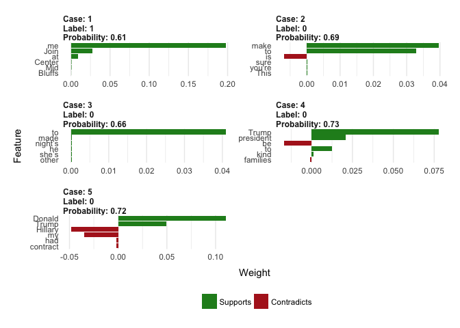
plot_features(corr_explanation)

Remember that Label == 1 means Donald Trump was the author of the tweet, otherwise it was Hilary Clinton. What does lime tell us? Funnily enough, it looks like presence of words like Donald, Trump, candidate and president indicates that Hilary was the author, whereas words like Hilary and me or my are indicative of Donald Trump. Sounds reasonable to me ;)
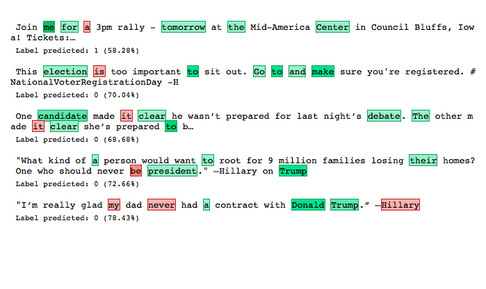
If you feel somehow ill at ease with this kind of presentation of model interpretations, try running plot_text_explanations() instead:
plot_text_explanations(corr_explanation)

It will give you a clearer view of support or contradiction of certain words for a given label, if you’re interested only in direction but not strength of this relationship.
Last, but definitely not least, it’s possible to run a shiny app to interactively explore text models. It’s not possible to run it in this blog, but all you need to do is run the following (single!) line of code to reveal its magic:
interactive_text_explanations(explainer)
Hope I managed to spread a bit of my love for lime! Again, big thanks to Thomas for a great job he did with this package! I can’t wait to see support for image data in R - but no pressure, the whole Twitter knows how busy you are :) Cheers!