My goal is to analyse how frequency of names found among Disney female characters changed over time in the US. Specifically, I want to see if the movie release had any impact on their popularity. For this purpose, I will use babynames dataset that is available on CRAN.
The idea for the exercise was inspired by Sean Kross’ blog post
short description of the dataset
from CRAN package description
The SSA baby names data comes from social security number (SSN) applications. SSA cards were first issued in 1936, but were only needed for people with an income. In 1986, the law changed effectively requiring all children to get an SSN at birth.
The dataset is quite simple, covering US baby name records from late 1800’s until 2014. It specifies whether a name is male or female, number of respective names in a given year and what proportion they constituted.
library(babynames)
baby <- babynames
baby$sex=as.factor(baby$sex)
summary(baby)
##       year      sex             name                 n
##  Min.   :1880   F:1081683   Length:1825433     Min.   :    5.0
##  1st Qu.:1949   M: 743750   Class :character   1st Qu.:    7.0
##  Median :1982               Mode  :character   Median :   12.0
##  Mean   :1973                                  Mean   :  184.7
##  3rd Qu.:2001                                  3rd Qu.:   32.0
##  Max.   :2014                                  Max.   :99680.0
##       prop
##  Min.   :2.260e-06
##  1st Qu.:3.910e-06
##  Median :7.390e-06
##  Mean   :1.407e-04
##  3rd Qu.:2.346e-05
##  Max.   :8.155e-02
installing packages
library(dplyr)
library(ggplot2)
quick data pre-prep
I assign each name to a separate dataframe.
ariel <- baby %>%
  filter(name == "Ariel", sex == "F")

belle <- baby %>%
  filter(name == "Belle", sex == "F")

jasmine <- baby %>%
  filter(name == "Jasmine", sex == "F")

tiana <- baby %>%
  filter(name == "Tiana", sex == "F")

merida <- baby %>%
  filter(name == "Merida", sex == "F")

elsa <- baby %>%
  filter(name == "Elsa", sex == "F")
Next, I create variables specifying the release date of a movie with character’s name.
# The Little Mermaid
ariel_release = 1989

# Beauty and the Beast
belle_release = 1991

# Alladin
jasmine_release = 1992

# The Princess and the Frog
tiana_release = 2009

# Brave
merida_release = 2012

# Frozen
elsa_release = 2013
plots
Finally, I plot the number of names for a given year. The arrows indicate when the movie was released, so that it’s easier to compare before and after trend. Additionally, I show the number of names and their proportion for a year proceeding and following the movie release. The numbers (and graphs!) say it all :-)
trends
Namely, the movie release indeed seems to have a positive impact on name popularity, at least short- , but often long-term. For example, Ariel, Belle showed much higher popularity that in pre-release days even a decade after the movie has been published.
Ariel
  ggplot(ariel, aes(x=year, y=n)) +
  geom_line(col="red") +
  xlab("") +
  ylab("") +
  ggtitle("Ariel") +
  geom_segment(aes(x = ariel_release, y = 0, xend = ariel_release, yend = 500), arrow = arrow(length = unit(0.1, "cm")))
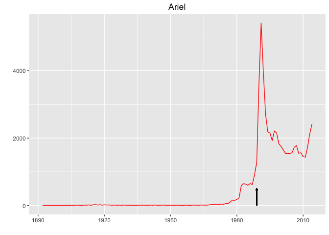
ariel %>%
  filter(year %in% c(ariel_release - 1,  ariel_release + 1))  %>%
  mutate(when = ifelse(year == ariel_release - 1, "1 yr before",
                      "1 yr after"))
## # A tibble: 2 × 6
##    year    sex  name     n        prop        when
##   <dbl> <fctr> <chr> <int>       <dbl>       <chr>
## 1  1988      F Ariel   910 0.000473441 1 yr before
## 2  1990      F Ariel  3604 0.001754975  1 yr after
Belle
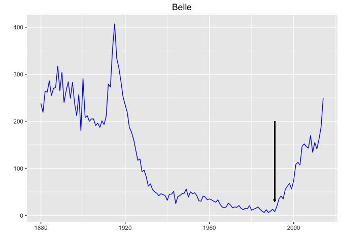
## # A tibble: 2 × 6
##    year    sex  name     n         prop        when
##   <dbl> <fctr> <chr> <int>        <dbl>       <chr>
## 1  1990      F Belle    13 6.330374e-06 1 yr before
## 2  1992      F Belle    19 9.480574e-06  1 yr after
Jasmine
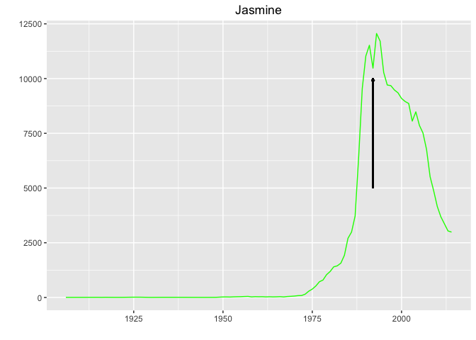
## # A tibble: 2 × 6
##    year    sex    name     n        prop        when
##   <dbl> <fctr>   <chr> <int>       <dbl>       <chr>
## 1  1991      F Jasmine 11523 0.005668207 1 yr before
## 2  1993      F Jasmine 12059 0.006118574  1 yr after
On the other hand, in case of Jasmine and Tiana, the positive effect of the Disney movie release on name’s popularity was rather short-term, although strong.
Tiana
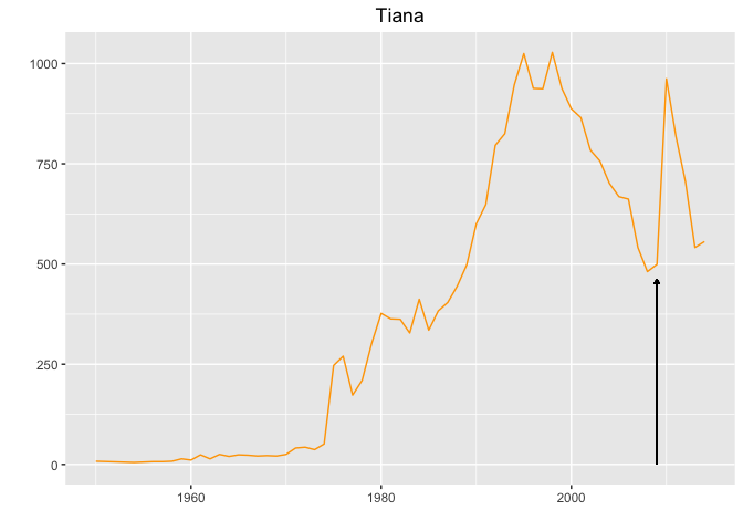
## # A tibble: 2 × 6
##    year    sex  name     n         prop        when
##   <dbl> <fctr> <chr> <int>        <dbl>       <chr>
## 1  2008      F Tiana   481 0.0002313058 1 yr before
## 2  2010      F Tiana   962 0.0004917941  1 yr after
Merida
Finally, it’s difficult to judge the long-term effect for names Merida and Elsa, as both movies have been released very recently, but at least a year following the release showed a remarkable jump in names’ popularity.
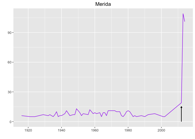
Here, the 1 year before and after comparison is not possible, as the movie was released in 2012 and no baby was called Merida in the US between 2002 and 2012. This still proves how powerful Disney movies can be!
tail(merida)
## # A tibble: 6 × 5
##    year    sex   name     n         prop
##   <dbl> <fctr>  <chr> <int>        <dbl>
## 1  1996      F Merida     8 4.174171e-06
## 2  2001      F Merida     5 2.526008e-06
## 3  2002      F Merida     5 2.533732e-06
## 4  2012      F Merida    19 9.831147e-06
## 5  2013      F Merida   109 5.681315e-05
## 6  2014      F Merida   101 5.210123e-05
Elsa
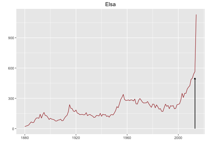
## # A tibble: 2 × 6
##    year    sex  name     n         prop        when
##   <dbl> <fctr> <chr> <int>        <dbl>       <chr>
## 1  2012      F  Elsa   540 0.0002794116 1 yr before
## 2  2014      F  Elsa  1131 0.0005834306  1 yr after
All in all, it goes to show that Disney movies are an important part of our culture that has the power to influence our lives in surprising ways :)